
Identifying Different Types of Historic Woodland with AI
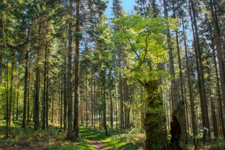
Image Source: Welsh Government
Using deep learning to detect different types of trees on historic maps.
Background
In October 2024, the Data Science Unit released the first AI Predicted Historic Woodland outputs on DataMapWales. This experimental dataset was created using a computer vision model and the Ordnance Survey (OS) Historic Landmark Map. It showed where woodland likely existed in Wales between 1843-1893 but did not distinguish between types of trees. Instead, each area was assigned a generic “woodland” label.
Knowing the potential location of ‘lost’ historic woodland is helpful for deciding which areas to target for woodland creation and regeneration schemes. Information about the type of woodland that existed, for example broadleaf or conifer species, can also be used to decide how suitable the area could be for replanting, depending on what type of tree was able to grow there previously.
This blog describes the next phase of work to develop a new multi labelled version of the dataset. These new outputs include information about the type of woodland that existed in each area, based on the symbols used on the historic maps.
Method: what types of trees can be identified?
Image segmentation models are a type of computer vision method which predict the location and identity of different objects in an image, based on a small sample of prelabelled images. The type of model used for this project was a deep learning convolutional neural network (Mask R-CNN) with a default resnet50_fpn architecture.
This is the same algorithm used to produce the first AI Predicted Historic Woodlands dataset. However, in this version of the dataset, the original labels the model was trained on are retained. This means that each predicted area is labelled as a specific type of woodland (rather than just assigned a generic “wood” label).
The OS Historic Landmark Map 25” County Series includes enough detail to distinguish between different types of trees on the map. The accompanying key indicates what general species of tree each stamp refers to and can be used create the woodland categories.
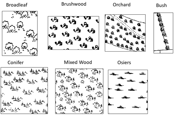
After consulting with Cadw, the Welsh Government historic environment service, and Natural Resources Wales, seven different types of woodland were used as labels. Figure 1 shows what type of map symbol was used to identify each woodland category.
Figure 1: The symbols associated with each type of woodland. The categories are Broadleaf, Brushwood, Orchard, Bush, Conifer, Mixed Wood, Osiers
The training data provided to the model also included “exclusion categories”. These “exclusion categories” were added based on common mis-predictions in an earlier model version where areas such as shorelines were incorrectly being predicted as woodland.
Adding labelled “Shoreline” and “Cliff like” objects to the training data reduced the number of times these features were mis-predicted as woodland. These predictions were then removed from the final outputs, leaving more accurate predicted areas of woodland.
For this version of the model, we increased the number of labelled objects of underrepresented woodland categories (Orchard and Brushwood) in the training data to improve the model performance for these groups specifically.
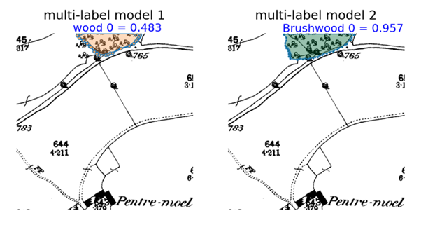
Figure 2 shows changes between the first and second versions of the model. For this example, the latest model, with the additional training data, has identified more brushwood correctly. The colours depict the confidence score of each prediction, with darker green representing high confidence and lighter shades representing lower confidence. The second version of the model made predictions with higher confidence, suggesting that training with the additional labelled objects has improved the quality of the model predictions.
Figure 2: Difference in model predictions of brushwood areas for the previous and current model.
The process of labelling the data and training the model was consistent with the method used to train the model for the AI Predicted Historic Woodland outputs. For more information on this, please refer to the previous blog
Evaluation: how good is the model at identifying different types of woodland?
The model performance was assessed using average precision. This metric combines precision and recall at different intersection over union thresholds (which measures how similar a predicted area is to a manually labelled area of woodland). The returned value represents the accuracy of the model detections compared to the manual labels.
The average precision for each individual category was calculated to assess how well the model performed across different types of woodland. A validation set of 351 labelled images (20% of the full labelled sample) was removed from the data before training. The predictions from the model were then compared to the manually labelled areas in these set of images. Table 1 shows the resulting average precision scores for each woodland category.
Table 1: Average precision scores across different woodland and exclusion categories
| Category | Average Precision |
|---|---|
| Broadleaf | 0.61 |
| Brushwood | 0.36 |
| Bush | 0.37 |
| Conifer | 0.73 |
| Mixed Wood | 0.56 |
| Orchard | 0.32 |
| Osiers | 0.53 |
The table shows that categories with distinct symbols, such as Conifer, have a higher average precision score compared to woodland types with similar symbols, like Orchard or Bush. The “mean average precision” of the model, calculated by taking the average of the average precision for each woodland category, is 0.5
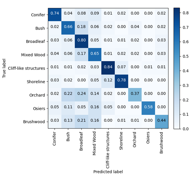
Figure 3 shows which categories are being predicted by the model compared to the expected woodland type (based on the manual labels). We count every time a manual object intersects with a predicted object with an intersection over union score greater than 0.3. This shows 80% of manually labelled Broadleaf areas overlap with the area of a predicted Broadleaf object. However, only 37% of manually labelled Orchard areas overlap with a predicted Orchard object; instead, these objects have also been predicted in the Bushes, Broadleaf and Mixed Wood categories.
Figure 3: Confusion matrix showing the different types of intersection between predicted and manually labelled woodland area
The differences between performance in these two categories could be due to appearance of the symbols. The main distinction between Orchard and Broadleaf areas is how the trees are stamped across the map. Orchard trees are generally located in a linear pattern, contained in smaller areas within a clear field boundary. Broadleaf often depicts much larger areas of continuous woodland instead. However, these two categories have very similar symbols, which could lead the model to incorrectly predicting Orchard areas as Broadleaf.
Also, there are more areas of Broadleaf, Mixed Wood and Bush woodland objects across Wales compared to Orchard areas. This might explain why there is a drop in performance for the minority class (Orchard) compared to the dominant classes as there are fewer labelled Orchard objects in the training and test datasets.
Process: creating a georeferenced dataset
To address the issue of a single area of woodland being assigned multiple labels, a series of post processing steps was used to simplify the output:
- The model predictions were converted to a polygon object and were georeferenced so they could be overlayed on the original historic maps.
- “Background” polygons (that overlapped with lots of other polygons, had a low confidence score and were square-shaped) were removed.
- In cases where two polygons overlapped, the intersecting area was removed from the polygon with the lower confidence score.
- Removed any polygons with an area <1 hectare.
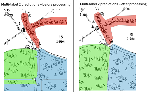
The image below shows the impact these steps have had on the model outputs, where it is clearer to see what woodland label has been assigned to each area after processing.
Figure 4: An area of Monmouth, before and after the post-processing steps area applied. The Conifer predicted area has been shaded in green, Mixed Wood predicted area has been shaded in blue and the Bush predicted area has been shaded in red
Limitations: what challenges are there?
The post-processing steps have improved the original model predictions however, there are still some inconsistencies with the final processed outputs. In cases where there are large areas with different tree symbols (particularly if the symbols are not clear or have limited field boundaries or other features), it is difficult for the model to predict the exact shape of different woodland in these areas.
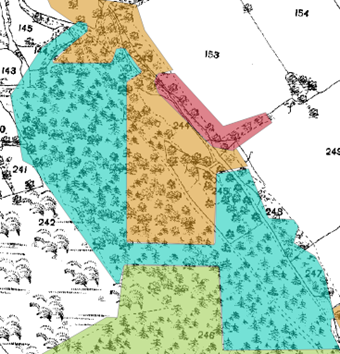
Sometimes, the predicted polygons of different woodland appear artificial, in unnatural squares or oblong shapes. We will continue to work on improving these outputs to minimize the effect of this for future versions and suggest considering all the predicted labels for the larger area if analysing locations where this occurs.
Figure 5: Example of a large area unnaturally split into different woodland types. The Conifer predicted area has been shaded in green, Broadleaf predicted area shaded in orange, Mixed Wood predicted area has been shaded in blue and the Bush predicted area has been shaded in red.
Wrap up: how should we use these outputs?
As the method to produce these estimates involves predictive modelling, there are risks to using them, where the model could predict the wrong label, or location, of woodland. Also, as explained, the shape of the final predicted polygons within larger areas might show differences after running the processing steps.
However, these outputs can instead be used to indicate the likelihood of certain types of woodland existing in Wales, for further investigation. They can be used as evidence, alongside other data sources, to show where regeneration efforts for specific types of woodland could be focused on the future.
Our next phase of work will look to apply this model to different versions (epochs) of the OS Historic Landmark Maps. This will test the feasibility of using the to identify areas of historic woodland at different points in time.